CTester
Handing Timeseries
We provide a Timeseries wrapper in the TimeSeries object which can be used
to atain information on a specified timeseries which can be passed normally as a pair OCHL or a custom pandas DataFrame.
Investigating the properties of investable timeseries has never been easier!
timeSeries = TimeSeries(client, data=pd.DataFrame())
A TimeSeries() requires a client object and an optional data input to calculate values from. The TimeSeries can be
filled with the appropriate data using a custom pass argument on data or via the standard download() function.
Each TimeSeries contains 5 internal variables these being:
Name |
Type |
Example |
Default |
Decription |
client |
Client |
Object |
None |
API client |
data |
DataFrame |
pd.frame |
None |
pd.DataFrame containing TimeSeries |
col |
String |
‘adj_close’ |
‘close’ |
Frame to Series pointer |
symbol |
String |
‘BTCUSDT’ |
None |
TimeSeries name |
interval |
String |
‘1d’ |
None |
Specifies timeseries interval |
Download
timeSeries = TimeSeries.download(symbol, interval)
This method passes data into the data field using the get_SpotKlines() to download OCHL data. It
requires the symbol and interval like the pre-mentioned funcion.
Requires: str: symbol, str: interval
Returns: Self
Slice
TimeSeries = TimeSeries.slice(col)
This method changes the col parameter of the TimeSeries object which dictates which column of the DataFrame passed in
data is used to make the singular TimeSeries for calculations.
Requires: str: col
Returns: self
Summarize
summary = TimeSeries.summarize(period=365, pct=False)
The summary() method returns a formatted DataFrame of summary statistics for the timeseries.
The pct parameter Specifies if the data passed is in price or percentage terms.
Return |
Volatility |
Sharpe |
Sortino |
MaxDrawDown |
Calmar |
Skew |
Kurtosis |
Requires: int: period, bool: pct
Returns: Pandas DataFrame
Linear Regression
est = TimeSeries.lin_reg(period=365)
This method returns the estimated annualised returns using Linear Regression.
Requires: int: period
Returns: float
Seasonality
szn = TimeSeries.seasonality()
This method returns a Panadas DataFrame with the average performed return by buissness month over the history of the timeSeries. This only works for intervals of ‘1d’ or more.
Requires: None
Returns: Pandas DataFrame
Autocorrelation
acf = TimeSeries.autocorrelation(period=365, lags=50, diff=False)
Returns autocorrrelation estimation across different lags as specified in the lag parameter. Autocorrelation differencing is possible by enabling the diff parameter.
Requires: int: period, int: lags, bool: diff
Returns: Pandas DataFrame
A.D. Fuller
adf = TimeSeries.adfuller(maxlags=5, mode='L', regression='ct')
This method performs the A.D. Fuller test using the statsmodels adf module and returns a Pandas DataFrame of relevant values as shown below. The regression input is directly related to the statsmodels implementation and represents the type of regression calculated.
ADF Value |
P-Value |
Lags |
N Obs |
C.V. 1% |
C.V. 5% |
C.V. 10% |
IC |
The A.D. Fuller test supports multiple price calculation methods, we have simplified the application of Logarithmic price transformation for the test through the mode parameter.
Acceptable Modes
Nominal (‘N’): Standard non-normalised price as downloaded via OCHL & sliced using col
Logarithmic (‘L’): Applies Logarithmic transformation to prices.
Requires: int: maxlags, str: mode, str: regression
Returns: Pandas DataFrame
Plotting Timeseries
plotter = Plotter(TimeSeries, path)
TimeSeries Plots
Plotter(TimeSeries).plot(period, mode, save)

This function enables plotting of a timeSeries and automates conversion into either Returns or Volatility via the mode parameter. This is a simplified way to see the basic (Level I) timeseries data.
Acceptable Modes
Nominal (‘N’): Plots the prices in standard nominal format.
Returns (‘R’): Plots the return as % gain/loss since period start.
Volatility (‘V’): Plots 7-day rolling standard deviation (Volatility) since period start.
Requires: int: period, str: mode, bool: save
Returns: Null
Quantile Plots
Plotter(TimeSeries).plot_qq(period, mode, save)
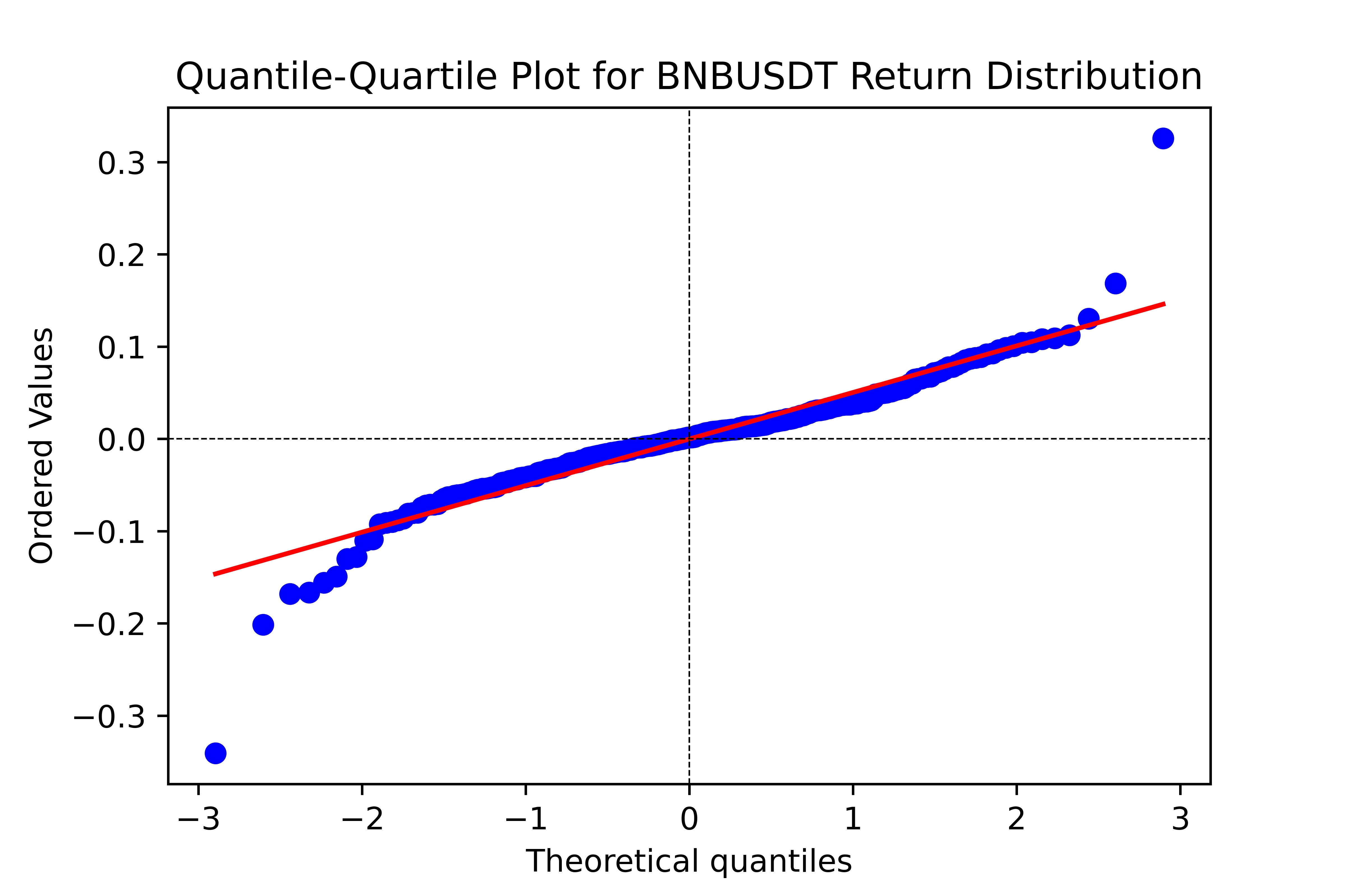
This function plots Quantile-Quantile with reference to normal distributions for quick analysis of the Return or Volatility distributions.
Acceptable Modes
Returns (‘R’): Plots the distribution of returns.
Volatility (‘V’): Plots the distribution of volatility.
Requires: int: period, str: mode, bool: save
Returns: Null
Seasonality Plot
Plotter(TimeSeries).plot_seasonality(save)
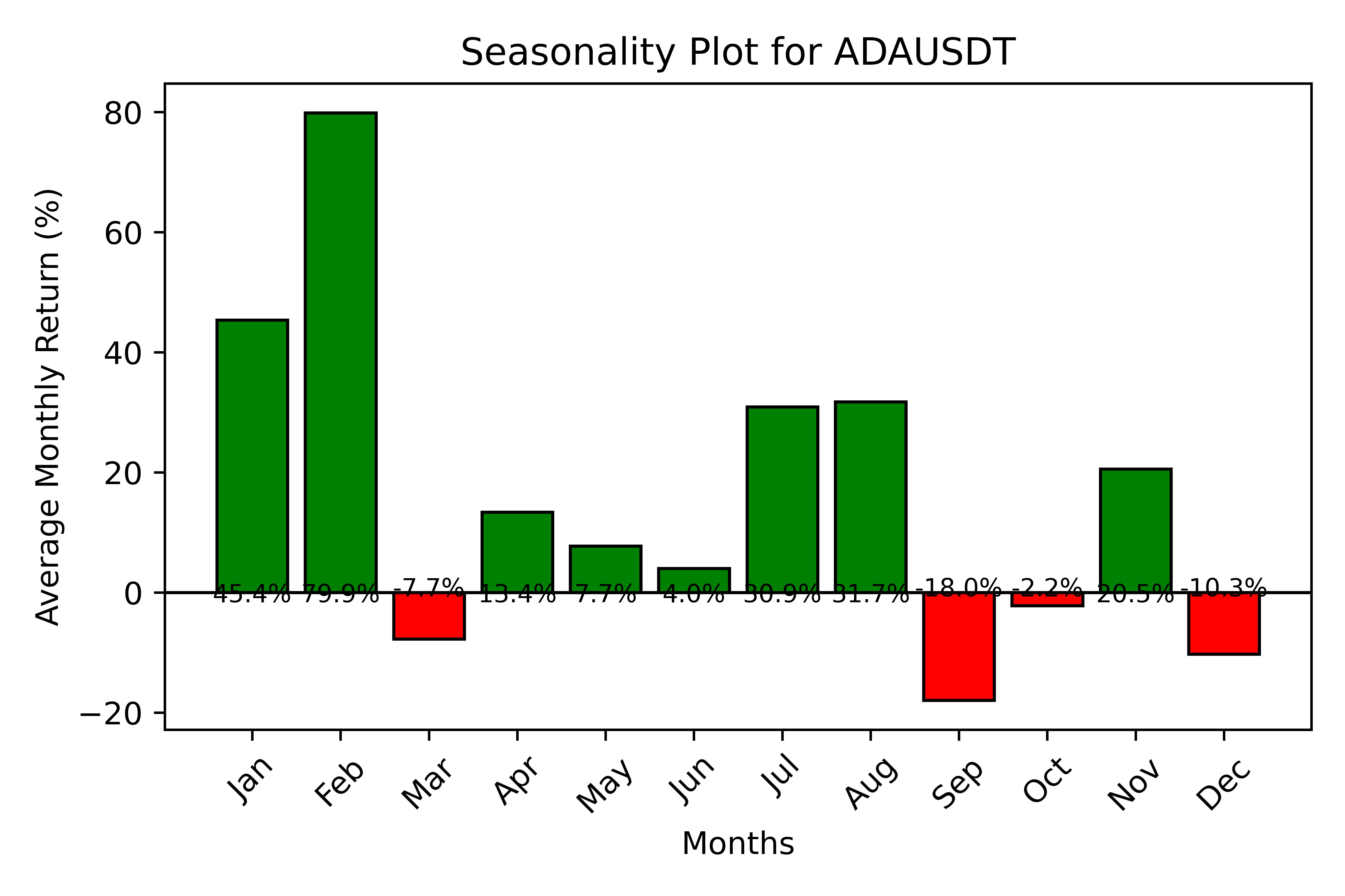
This function plots the seasonality statistic, i.e. the average performed monthly return of the timeseries. It shows a matplotlib barplot with relevant information which can be saved.
Requires: bool: save
Returns: Null
Autocorrelation Plot
Plotter(TimeSeries).plot_acf(period, lags, diff, save)
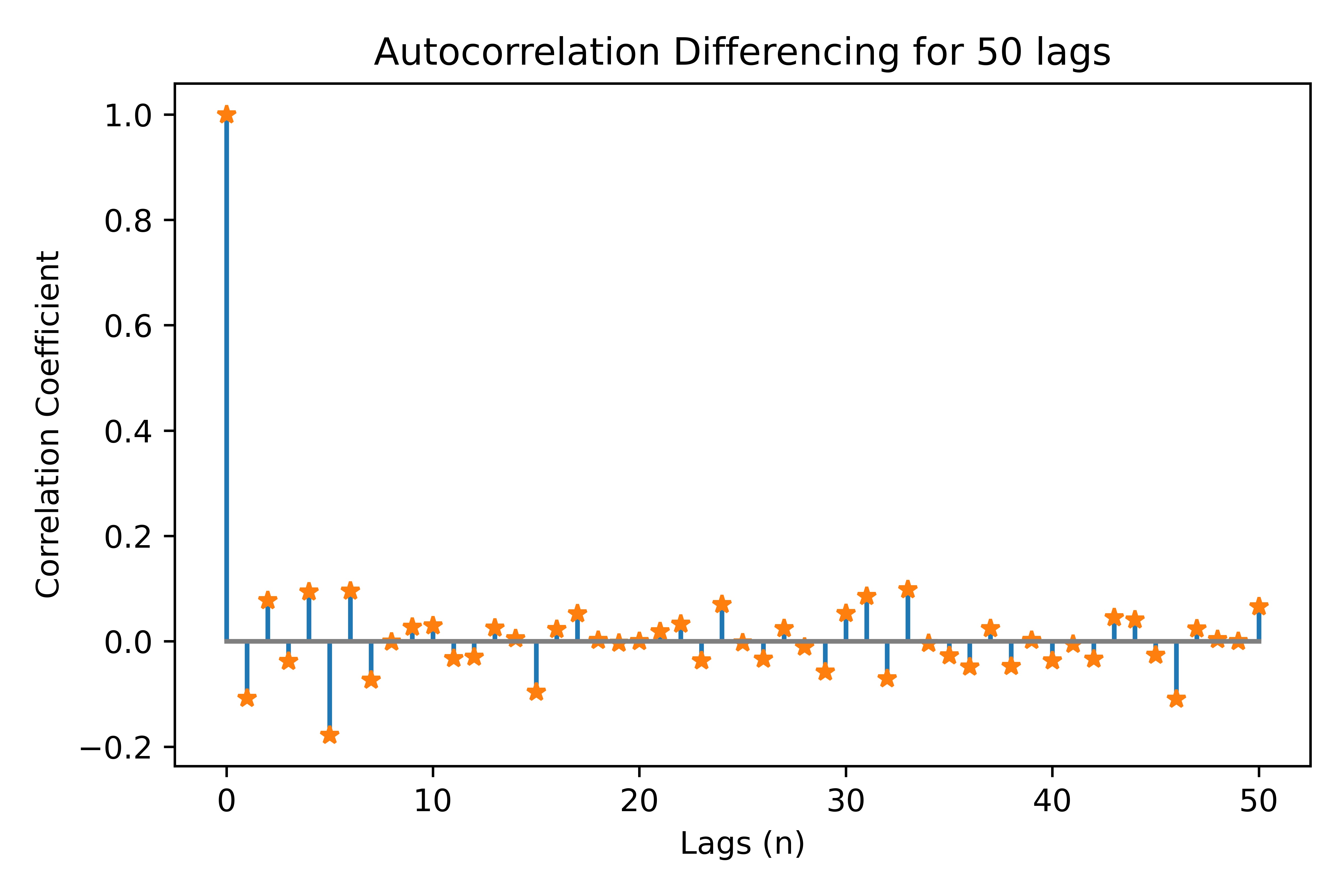
This function plots the autocorrelation for specified lags; it can plot differenced autocorrelation by enabling the diff parameter.
It shows a matplotlib stemplot which can be saved.
Requires: int: period, int: lags, bool: diff, bool: save
Returns: Null
Benchmark Plot
Plotter(TimeSeries).benchmark(benchmark, period, delta, save)
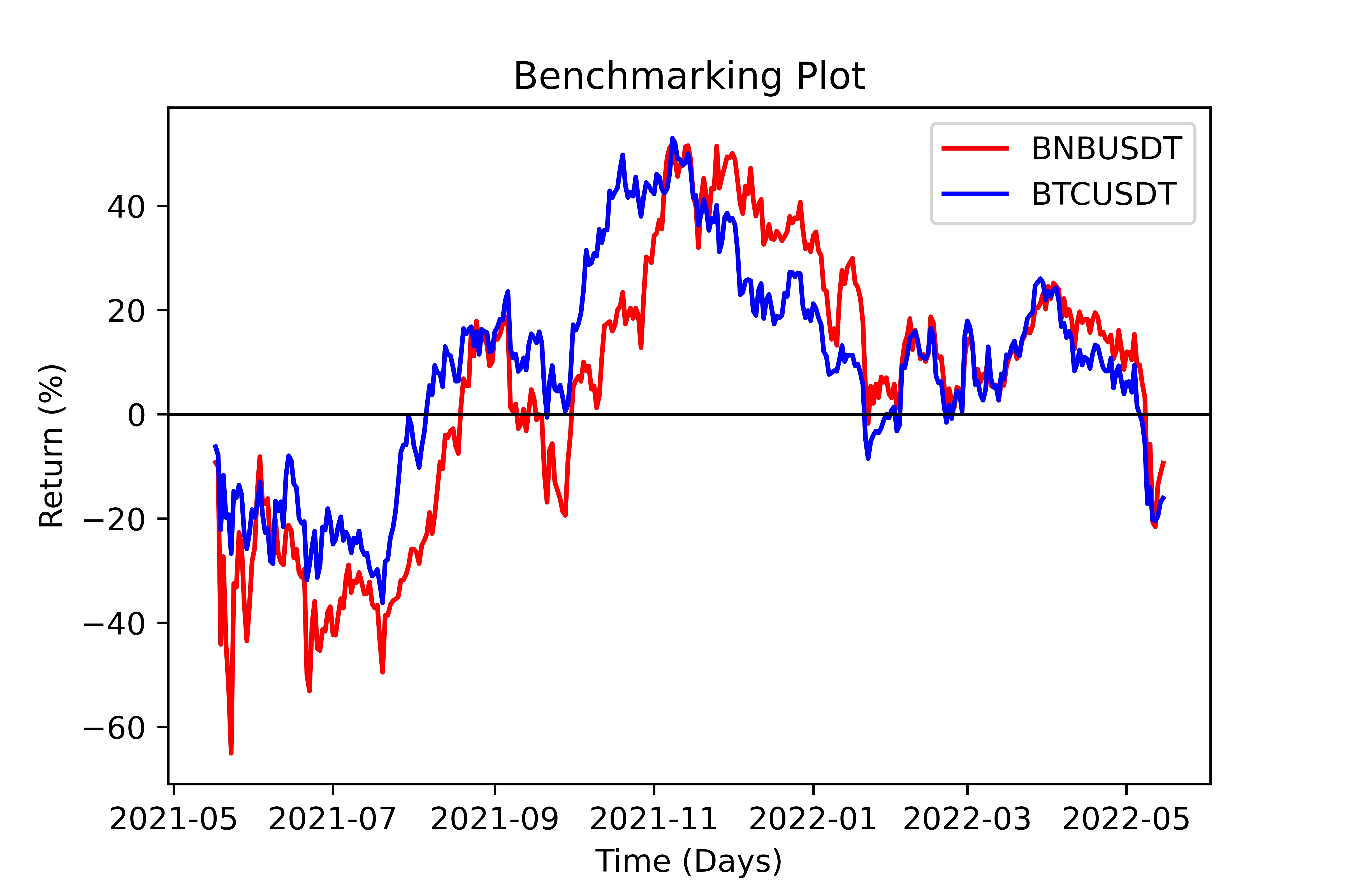
This function plots the specified timeseries against a benchmark timeseries. It may return the 1:1 spread (delta) between the two timeseries via
the delta parameter. It shows a matplotlib lineplot which can be saved.
Requires: str: benchmark, int: period, bool: delta, bool: save
Returns: Null
Handling Portfolios
We have packaged additional functionality through the Portfolio object which enables users to calculate performance analyses on portfolios.
Through this object, it is possible to define and parameterise portfolio level quantitative data-points. This is also connected to the portoflio backtesting suite
via the MonteCarlo engine.
portfolio = Portfolio(client, symbols, weights, interval, download)
In the above statement, there is a simple definition of a portfolio, it contains a list of symbols and coresponding weights, a timeseries interval and a download check.
First, the symbols need always get passed and represent the basic parameter of the portfolio. Second, the weights parameter needs to be an array of floats summing to 1; however,
if it ommitted it is automatically set to equal weighting across symbols. Third, the interval paarameter represents the timeseries interval for the download, if the donwload parameter is
False then interval is ommitted. In the cases where download is false, the weights & interval may be ommitted.
The input format for the data parameter is a Pandas DataFrame with each column being a select single-variable timeseries of each asset, with the columns being the tickers.
Name |
Type |
Example |
Default |
Decription |
client |
Client |
Object |
None |
API client |
symbols |
str array |
[‘ADAUSDT’] |
None |
pd.DataFrame containing TimeSeries |
weights |
float array |
[0.3, 0.7] |
None |
Frame to Series pointer |
interval |
String |
‘1d’ |
None |
Specifies timeseries interval |
download |
bool |
True |
True |
Download timeseries data or not? |
Calculte Equity Curve
eqCurve = Portfolio.equity_curve(period=365)
This method returns the cummulative return (‘Equity Curve’) of the calculated portfolio by parsing data against weights.
It returns a timeseries DataFrame with timestamps and return values.
Requires: int: period
Returns Pandas DataFrame
Load Data
Portfolio = Portfolio.load_data(data)
This method enables us to bypass the data download phase of the portfolio by loading the data object discretely.
Requires:: Pandas DataFrame: data
Returns: obj: Portfolio
Summarize
summary = Portfolio.summarize(period=365)
This method returns a number of summary statistics of the specified Portfolio timeseries which can help in quantitative analysis. The return fields
can be seen in the table below. Expected values represent calculations derived from the Mean. The Sortino, Draw Down, Calmar, Skew and Kurtosis, measures
are derived from the full timeseries. The Performed values (Return, Vol, Sharpe) are calculated using the period parameter
(i.e. ‘PerformedReturn’ for a period of 365 is 1YR return)
Weights |
Exp. Ret |
Exp. Vol |
Exp. Sharpe |
Sortino |
MaxDD |
Calmar |
Return |
Vol. |
Sharpe |
Skew |
Kurtosis |
Requires: int: period
Returns Pandas DataFrame
Long Only Portfolio Backtesting
mcEngine = MonteCarlo(client, symbols)
The Monte Carlo Engine provides an efficient way for us to run Simulation of portfolio performance through shifting the
weights parameter. Through this wrapper we can view certain optimisation functionality aimed at Long-Only Portfolios.
Requires: obj: client, arr of str: symbols
Returns obj: MonteCarlo
Run Simulation
mcEngine = mcEngine.run(runs=5000)
This method enables users to backtest the historic performance of randomly weighted portfolios of the specified symbols. The outcome of this method
is a filled Pandas DataFrame containing the timeseries information calculated via summary() in the timeseries package. It also includes an
annualised expected calcuation of returns, volatility and sharpe by extrapolating the returns distribution.
Requires: int: runs
Returns obj: MonteCarlo
Efficient Frontier
mcEngine.eft(mode='E')
This method returns the top-5 results calculated through run() as per the Efficient Frontier Theory; that being sorted by Sharpe ratio.
We provide the mode parameter such that the sorting may be done via exppected returns or 1 year performed returns.
Acceptable Modes
Expected (‘E’): Returns the top-5 portfolios based on expected sharpe ratio of all timeseries data.
Performed (‘P’): Returns the top-5 portfolios based on 1 year performed sharpe.
Requires: str: mode
Returns Pandas DataFrame
Pairs Trading
pair = CSuite.Pair(client, symbols, interval, download)
We include a specialised Pairs Trading handler that allows users to easily analyse pair trading and other spread based startegies. A Pair object
contains a customisable data structure of DataFrame type, alongside a client, symbols and, an interval string.
It is initailized with the download parameter which specifies whether the data filed is filled using the batch_historic function.
Requires: obj: client, arr str: symbols, str: interval, bool: download
Retuns: obj: Pair
The Spread
spread = pair.get_spread()
A Pair contains a spread which is the difference in daily closing prices between the two timeseries. Since this in itself is a timeseries, it is a child class
of the timeseries object and can utilise functions like summarize or adfuller. The Spread can be created through the Pair object:
Note
The Spread can be plotted using the Plotter
Requires: None
Returns: obj: Spread
Johansen test
spread.johansen(maxLags=20)
Requires: int: maxLags
Return: null
VCEM Forecast
forecast = spread.VCEM_forecast(periods, lags, coints, backtest=False, confi=0.05, determ='ci')
The VCEM_forecast method enables users to easy get a forward prediction of a cointegratable spread using the Vector Error Correction Model. It returns a timeseries of the
upper, lower and, mid band estimates of the expected value of the spread over the forecast period (periods). The forecast is only possible through the lags and cointegration parameters
which are derived from the the Johansen Test (johansen()).
The backtest option enables users to quickly verify data against the timeseries itself. If set to True, the forecast will be calculated on the timeseries excluding the latest
periods datapoints. Then that forecast can be compared to the timeseries manually.
The final two parameters namely, confi and determ specify the VCEM setup, the first is the confidence interval, set at 5% and the second, the deterministic terms
which are derived from the statsmodels VCEM function which we use here.
This setting defauls to ‘Constant with Cointegration Relation’.
Requires: int: periods, int: lags, int: coints, bool: backtest, float: confi, str: determ
Returns: DataFrame: forecast